A plastic injection molding cost estimator is most valuable before a design is frozen, because it converts engineering choices into a comparable business case. The estimator should not merely predict a unit price. It should show how tooling investment, part weight, cycle time, cavity count, reject rate, secondary operations and lifetime demand affect margin, cash exposure, payback and production capacity. Used this way, the model identifies the few design changes that can improve return on investment before a mold becomes expensive to modify.

The right early-stage question is not 鈥淲hat will this part cost?鈥?but 鈥淲hich assumptions control the economics, and what must be validated next?鈥?A useful estimate therefore presents a range, records its assumptions and compares several scenarios. A supplier quotation can later replace assumptions with geometry-specific costs, but the estimator gives product, engineering and procurement teams a common financial language before requesting quotes.

What should an injection molding cost estimator calculate?

A practical estimator separates recurring cost from one-time investment. Recurring cost includes resin, machine time, direct labor, scrap, inspection, packaging and secondary processes. One-time investment includes the mold, fixtures, gauges, automation, qualification and sample iterations. Keeping these groups separate matters because the same unit-cost result can hide very different cash requirements and risks.

The basic recurring-cost equation is:

Good-part cost = material cost + conversion cost + labor + secondary operations + quality and packaging + allocated nonrecurring cost.

Material cost should use the total shot weight rather than finished part weight alone. The shot may include runners, sprues and process loss. Conversion cost is normally calculated from the fully loaded machine hourly rate, cycle time and number of acceptable parts produced per cycle. Tool cost may be shown separately for cash planning and allocated across an expected quantity for product-margin analysis.

Estimator input	What it represents	Early decision it supports
Part and runner weight	Total resin consumed per shot	Wall, gate and runner optimization
Resin price and yield	Material cost per good part	Grade selection and scrap sensitivity
Cycle time	Seconds of press capacity per shot	Cooling, wall thickness and automation
Machine rate and tonnage	Cost of the required molding cell	Projected area and press selection
Cavity count	Parts made during each cycle	Tool investment versus throughput
Tooling and qualification	Upfront program investment	Payback, cash flow and launch timing
Lifetime demand	Expected saleable parts over the program	Tool class, cavitation and amortization
Secondary operations	Work performed after molding	Part consolidation and automation

Why a precise-looking estimate can still be wrong

An estimator can produce a result to four decimal places even when its inputs are uncertain. Early CAD may not define the resin grade, tolerance scheme, cosmetic standard, gate location or annual volume. Estimated cycle time may ignore cooling limitations, and a nominal scrap percentage may exclude start-up loss or an unstable assembly operation. Precision in the output does not remove uncertainty in the assumptions.

A better model assigns an evidence level to every major input. 鈥淜nown鈥?values come from released requirements or contracted prices. 鈥淐alculated鈥?values come from geometry and process models. 鈥淏enchmark鈥?values come from comparable programs. 鈥淯nknown鈥?values require a range. This simple classification prevents a benchmark resin price and an approved supplier price from being treated as equally reliable.

Use three scenarios instead of one forecast. The base case should represent the most likely design and demand. The downside case should combine lower volume, a longer cycle, more scrap and higher qualification cost. The improvement case should include only changes that engineering believes are feasible, such as a thinner uniform wall or elimination of a secondary operation. The spread between scenarios is often more useful than the base-case number.

Step 1: define the commercial baseline before entering process data

ROI cannot be optimized without a commercial baseline. Record the selling price or internal transfer value, expected annual demand, program life, launch date, forecast confidence and required gross margin. If the component replaces another process, also record the current purchase price, assembly labor, defect cost, inventory and warranty exposure. Injection molding may create value through part consolidation or consistent quality even when its isolated piece price is not the lowest.

Demand should be modeled by year rather than as one lifetime total. A program expecting 500,000 pieces over five years may ramp slowly, peak in year three and decline afterward. That pattern changes the payback date, capacity requirement and risk of investing in a high-cavity tool. The same lifetime volume with a faster first-year ramp may justify more cavities or a production mold immediately.

Separate demand from order quantity. Allocating a mold over 500,000 expected parts does not mean the buyer will order 500,000 parts at once. Tooling payment terms, minimum order quantity, safety stock and batch setup costs determine early cash consumption. A profitable lifetime model can still create a working-capital problem during launch.

Step 2: build the material-cost input from the complete shot

Material cost per good part starts with part mass, runner mass, cavity count, resin price and yield. The calculation should distinguish reusable regrind from material that cannot return to the process. Medical, optical, electrical or highly cosmetic applications may restrict regrind even when a general estimator assumes that runners have recovery value.

A useful simplified equation is:

Material cost per good part = [(shot weight 脳 resin price) 梅 cavities] 梅 first-pass yield.

The estimator should then test material price volatility. A five- or ten-percent change in resin price may matter more than a small tooling discount when the part is heavy and annual demand is high. Conversely, resin negotiation has limited value when machining time, complex inserts or manual finishing dominate the cost. A cost breakdown tells procurement where negotiation effort can actually affect ROI.

Material substitutions require an engineering comparison, not a price-only assumption. A lower-cost resin can change shrinkage, cooling time, mold steel requirements, draft, wall thickness, dimensional stability or product life. The model should capture the system effect rather than multiplying the current part weight by a cheaper price per kilogram.

Step 3: convert cycle time and machine rate into capacity cost

Machine cost per good part is typically calculated as the machine hourly rate multiplied by cycle time, divided by 3,600 seconds and then divided by the number of good parts produced per cycle. The hourly rate should match the required press tonnage and cell configuration. A generic rate can be misleading when the design requires a larger press, hot-runner controller, dryer, robot, temperature-control unit or insert-loading station.

Machine cost per good part = (hourly cell rate 脳 cycle seconds 梅 3,600) 梅 good parts per cycle.

Cycle time is often one of the strongest recurring-cost levers. Cooling commonly consumes a large share of the molding cycle, so excessive wall thickness can increase both resin consumption and machine time. The injection molding DFM guide explains why uniform walls, practical draft, ribs and well-designed bosses can reduce manufacturing difficulty before tooling begins.

The capacity check should run beside the cost calculation. Parts per hour, planned uptime, shifts and annual working days determine whether the assumed mold can satisfy peak demand. A low estimated unit price has little value if the cell cannot meet the launch schedule. Capacity utilization also affects the economic value of adding cavities: more cavities can lower conversion cost, but the extra tool investment may be unnecessary when demand is modest.

Step 4: compare cavity strategies instead of assuming more is better

Cavity count creates a central tradeoff. A multi-cavity mold produces more pieces per cycle and can reduce machine cost per part, but it generally requires more mold steel, machining, cooling, hot-runner capacity and validation. It may also require a larger press. A cost estimator should compare one-, two-, four- and higher-cavity concepts using the same demand forecast.

For each cavity option, calculate upfront tool cost, expected cycle time, press requirement, annual capacity, tooling amortization and payback. Also include the cost of spare inserts or critical hot-runner components when downtime would be expensive. A four-cavity option is not automatically superior to a two-cavity option if demand is uncertain and the additional investment pays back late in the program.

Geometry can limit the cavity strategy. Side actions, unscrewing mechanisms, tight tolerances, large projected area and difficult cooling layouts consume mold space or complicate balancing. The estimator should flag these features rather than treating cavity count as a free input. The earlier article on injection mold cost drivers provides a deeper breakdown of the tooling features that affect a formal mold quote.

Step 5: model tooling as both investment and technical asset

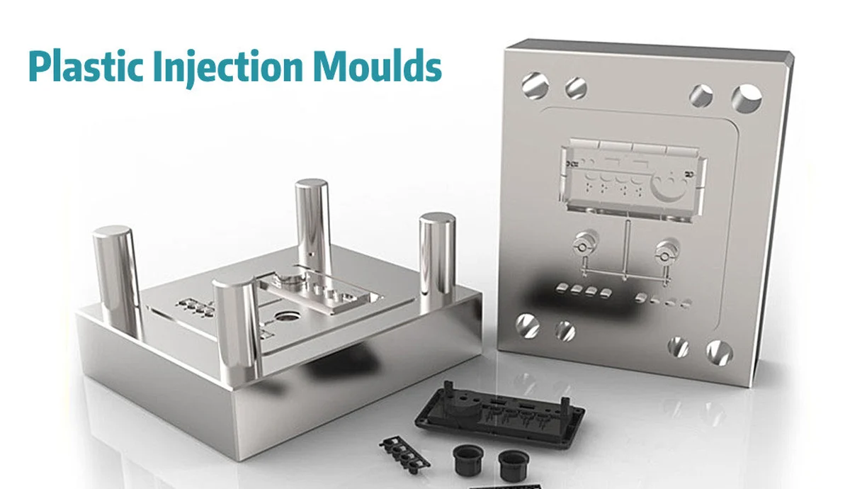
Tooling cost should include more than the mold purchase price. Add DFM and mold-flow work when required, sample rounds, fixture and gauge construction, qualification, texture approval, spare components, shipping, installation and any transfer documentation. A low initial mold quote can understate total program investment when these items are excluded.

Tool life should be expressed in shots and translated into saleable parts using cavity count and expected yield. The resin, glass loading, surface finish, maintenance plan and mold construction influence useful life. If forecast demand approaches the assumed mold life, add maintenance events or replacement inserts to the model. Amortizing one tool across a volume that requires two tools overstates ROI.

Ownership and transferability also have financial value. The purchase agreement should identify ownership of mold components, CAD, drawings, process settings and dedicated gauges. It should define storage, preventive maintenance, insurance, access and transfer conditions. These controls do not necessarily reduce the initial estimate, but they protect the investment if production must move.

Step 6: include the costs that simple calculators often omit

Simple estimators commonly stop at material, machine time and mold amortization. A B2B sourcing model should also evaluate setup and changeover, color changes, insert loading, trimming, printing, painting, welding, assembly, inspection, testing, packaging and freight. These costs may be quoted per part, per batch or per labor hour, so the model must avoid double counting overhead already included in the machine rate.

Quality cost deserves a visible line. Include start-up scrap, routine reject rate, inspection labor, gauge calibration, destructive testing and expected rework. For critical parts, qualification may require capability studies, first-article reports, material traceability or approved process windows. A lower piece price may not create a better ROI if it depends on higher inspection or failure risk.

Logistics and inventory should be included when comparing sourcing regions or batch sizes. Freight, duties, packaging density, transit inventory, minimum order quantity and buffer stock affect landed cost and cash. The OEM plastic parts supply continuity guide explains how tooling, materials, capacity and recovery planning influence total supply risk beyond the quoted unit price.

Step 7: calculate ROI, payback and break-even volume

ROI should use the economic benefit created by the investment, not just the reduction in unit cost. For a new product, contribution per part can be modeled as selling price minus variable manufacturing, logistics and selling costs. For a process conversion, annual benefit may include unit savings, eliminated assembly labor, lower scrap, reduced warranty cost and inventory reduction.

Simple project ROI = (cumulative net benefit 鈭?initial investment) 梅 initial investment.

Payback volume = initial investment 梅 contribution or savings per part.

For example, consider a hypothetical component with $28,000 in tooling and qualification cost. If injection molding creates $0.70 of net benefit per saleable part compared with the baseline, simple payback occurs at 40,000 parts. If the downside scenario reduces benefit to $0.40 per part, payback moves to 70,000 parts. The second number may be more important if forecast confidence is low.

Break-even analysis should compare alternatives on the same basis. A low-investment tool may have a higher piece price, while a production tool requires more capital but lowers recurring cost. The break-even quantity between two options is:

Break-even quantity = difference in upfront cost 梅 difference in variable cost per part.

If Tool A costs $12,000 and produces parts for $1.20, while Tool B costs $32,000 and produces parts for $0.70, Tool B recovers its additional $20,000 after 40,000 parts. The decision still depends on timing, forecast confidence, capacity and tool-life requirements; break-even volume alone does not measure risk.

Step 8: use sensitivity analysis to find the highest-value DFM work

Sensitivity analysis changes one input at a time and records the effect on payback or gross margin. Test part weight, runner weight, resin price, cycle time, cavities, yield, tool cost and demand. Rank the inputs by financial impact. The largest controllable variables become the priorities for engineering and supplier discussion.

A tornado chart or simple ranked table can make the result visible to nontechnical stakeholders. If cycle time has the largest effect, focus on wall thickness, cooling, ejection and process stability. If material dominates, focus on weight, runner design and grade selection. If tooling dominates only in the downside-volume case, consider a bridge tool or staged investment rather than over-optimizing a few cents of machine time.

The estimator should preserve scenario versions. Save the original baseline, the DFM proposal and the supplier-reviewed model. Record who changed each assumption and why. This prevents an optimistic cycle-time estimate from silently becoming a committed budget and gives sourcing teams a clean basis for comparing quotations.

Worked example: turning an estimator into an early ROI decision

Assume a team is evaluating a molded housing with a forecast of 60,000 parts per year for four years. The initial concept uses 85 grams of resin, a cold runner, a 38-second cycle, two cavities and a manual label. The estimator shows that material and machine time dominate recurring cost, while the two-cavity tool pays back comfortably in the base case but slowly in the downside-volume case.

A DFM review proposes three changes: reduce average wall thickness while maintaining rib-supported stiffness, redesign the gate and runner, and mold the identification detail into the part. The updated estimate uses 74 grams per part, a 34-second cycle and no manual label. Tooling becomes slightly more expensive because of the revised surface detail, but recurring cost falls on every good part.

The decision should be approved only after checking technical consequences. Thinner walls must still fill reliably and meet impact requirements. Molded identification must remain legible within the selected texture. The supplier should validate cycle time and yield during sampling. The estimator identifies a promising ROI direction; DFM, simulation, prototyping and trial data convert that direction into a controlled production plan.

How to reconcile an estimate with supplier quotations

A supplier quote should not be compared with the estimator as one total number. Map each quote line to the model: resin grade and price basis, net and shot weight, mold specification, cavity count, press tonnage, cycle time, yield assumption, labor, secondary operations, inspection, packaging, Incoterm and annual volume. Differences reveal which assumptions need clarification.

Two quotations can use different commercial structures. One may include mold maintenance in the unit price; another may charge maintenance separately. One may quote ex-works production; another may include export packaging. One may assume a family mold or shared press allocation that affects scheduling. A normalized comparison is more reliable than selecting the lowest displayed unit price.

Send suppliers a consistent RFQ package containing 3D CAD, dimensioned drawings, material specification, finish requirements, critical characteristics, annual and lifetime volumes, batch sizes, quality documentation, packaging and delivery location. The engineer鈥檚 sourcing checklist explains the technical information needed for a quote-ready package.

When should the estimate be updated?

The cost model should be updated at defined development gates. At concept stage, it supports process selection and rough investment planning. After DFM, it should reflect feasible geometry, material and mold concepts. After the supplier quote, it should replace benchmarks with quoted assumptions. After T1 samples, it should use measured part weight, cycle time and observed defects. After pilot production, it should include demonstrated capacity and first-pass yield.

This progressive refinement prevents the early estimator from being treated as a permanent standard cost. It also creates a learning loop: the difference between estimated and measured results improves future projects. The CAD-to-functional-part guide shows how prototyping, DFM, tooling and validation fit into a faster but controlled launch sequence.

Injection molding estimator checklist for B2B teams

• State whether every input is known, calculated, benchmarked or unknown.
• Use part weight plus runner and process loss, not finished weight alone.
• Match machine rate to projected area, clamp force and required auxiliaries.
• Compare cavity strategies using tool cost, capacity and program demand.
• Separate tooling cash outlay from accounting amortization.
• Include sampling, gauges, qualification, maintenance and replacement risk.
• Model secondary processes, quality, packaging, freight and inventory.
• Run base, downside and improvement scenarios.
• Calculate payback volume as well as unit cost.
• Use sensitivity analysis to prioritize DFM work.
• Normalize supplier quotes against the estimator鈥檚 assumptions.
• Replace assumptions with measured data after trials and pilot production.

What is the best way to optimize ROI early?

The best early ROI improvement is usually not a blanket reduction in tooling price. It is the removal of a recurring cost or risk that affects every future part. Uniform walls can reduce resin and cooling time. Removing an undercut can simplify tooling and increase feasible cavitation. Consolidating an assembly can eliminate components, labor and failure points. A stable process can reduce scrap, inspection and delivery risk simultaneously.

A plastic injection molding cost estimator should therefore function as a decision model, not a price oracle. The model is successful when it makes assumptions visible, identifies the most valuable design changes and prepares the team for a more accurate supplier quotation. It should be retired or recalibrated when real DFM, sampling and production data become available.

Discuss your plastic part ROI with DJMolding

DJMolding supports B2B customers with plastic part DFM, mold development, injection molding and production planning. Share your CAD files, material requirements, expected volumes, quality needs and target economics to receive a project-specific review. Contact DJMolding to discuss how design, tooling and manufacturing choices can improve ROI before your product reaches mass production, or explore more injection molding resources across the DJMolding website.